.jpg?hsLang=en-us)
A Microclimate and Chill Accumulation Case Study
Chill is required for leaf and flower bud development in many fruit and nut trees. "Industry research has determined a lack of sufficient hours below 45° F affects the nut crop that develops in the spring. There can be poor fruit bud development, delayed or strung out bloom and poor overlap with pollinators". The ability to set a crop can be affected as well as maturity timing resulting in need for multiple harvests. As we enter spring and the end of chill accumulation, we have many customers wondering why their chill hours can differ so much from the regional weather stations.
In some cases, the difference in chill in their own orchard can even be more pronounced than between their own stations and a neighbor’s.
The reasons for this can be attributed to
- Microclimate variation and
- Temperature fluctuation sensitivities between chill models.
A Chill Accumulation Case Study in Pistachios
One of our pistachio-growing customers that has five weather stations across their property noticed last year that there were some differences between their chill hours and chill portions.
Two weather stations had accumulated chill hours in the 300 range, while the other two had over 500 chill hours accumulated. Meanwhile, their chill portions across all stations were sitting at approximately 35.
How do chill hours accumulate?
Chill hours are the number of hours when the temperature drops below 45 °F, or is between 32 - 45 °F, depending on the model you use.
Let’s look at the temperature over time at two of their weather stations.
Station A has accumulated 326 chill hours, and 37 chill portions and Station B has accumulated 589 chill hours, and 39 chill portions.
-1.png?hsLang=en-us)
Figure 1. Temperature at two different weather stations in the same orchard
You can see that, although the weather stations track each other quite closely on average, Station A tends to have warmer nights than Station B. In mid-November, when the temperature for A hovers around the 45 °F threshold, fewer chill hours accumulate compared to B, which has nighttime temperatures of approximately 35 °F.
With this in mind, it is important to remember that chill is cumulative which is why small differences can add up significantly over time.
Microclimates - Customer Case Study
Last season, one of our grower customers asked us to analyze the variation in chill accumulation he was seeing between two of his weather stations.
Below shows a chill hours accumulation heat map (Figure 2). This heat map is calculated based on the climate data being collected from our networked aerosol mating disruption dispensers, which track temperature, relative humidity, and barometric pressure in-canopy.
From this map, you can see that Station B is in an area that is cooler, and has accumulated more chill hours.
Station A is in an area that is warmer, and therefore has accumulated less chill hours.
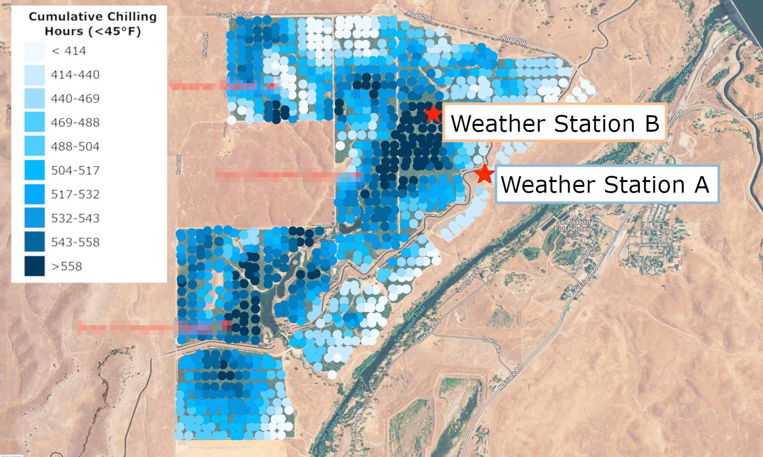
Figure 2. In-canopy sensor chill hours accumulations
Many factors can affect air temperature. Some of these include
- Elevation
- Row orientation
- Distance from a body of water
- Distance from east vs. west facing rock formation soil type
The south-east side, where Station A is located, is at a lower elevation and close to a river which leads to warmer temperatures during this time of season (Figure 3). In addition, we can tell from looking at satellite imagery (Figure 4), that Station B might be impacted by vegetation cover. The green areas, have denser winter-time vegetation and have understandably accumulated more chill.
The yellow areas, which are sparser, have accumulated less.
Vegetation can affect air temperature by processes such as evapotranspiration, respiration and impacting the heat transfer between the ground and the air.

Figure 3. Elevation map
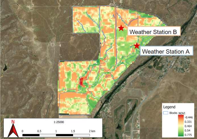
Figure 4. NDVI satellite imagery. Green areas show regions with denser winter time vegetation while red areas are more sparse.
Chill portions
As stated above, chill is cumulative and therefore small variations in microclimates can lead to large differences in chill over time. Although we can see this in the large variation in chill hours, differences in chill portions are less pronounced. The Dynamic Model, which is used to calculate chill portions, was developed based on experiments where plants were introduced to different temperature cycles. Two features of the Dynamic Model dampen the effects of temperature variation.
- Heat can ‘undo’ chill
- Not all cold temperatures contribute equally to chill
The Dynamic Model uses a two step process for chill accumulation. In the first step, cold temperatures lead to an intermediate product being formed (not seen in the output) while warm temperatures can destroy this product (Figure 5). However, once a certain amount of intermediate product is accumulated, it is converted to a permanent product which is seen in the model output as a ‘chill portion’ which cannot be destroyed.
Essentially, heat can ‘undo’ the chill, which is not possible in the chill hours model.
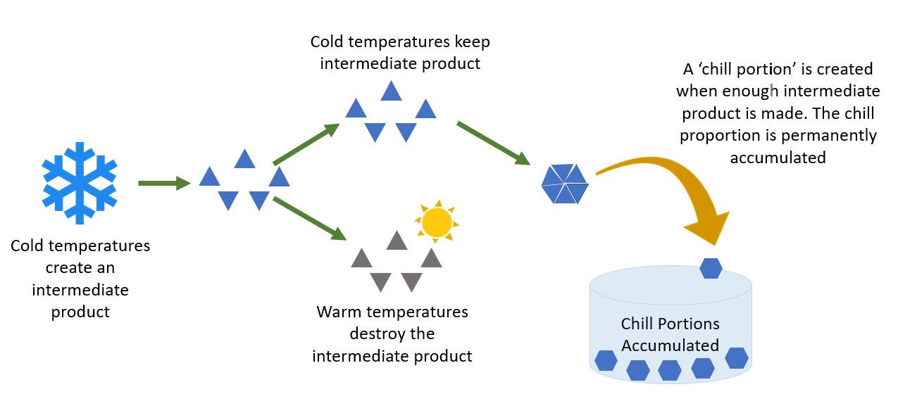
Figure 5. Dynamic chill model (chill portions)
The second feature of the Dynamic Model (portions), that dampens the effects of temperature variation, is how not all cold temperatures have the same contribution to chill accumulation. Temperatures in the 43 - 47 °F range will contribute the most to chill portions, while temperatures from 32 - 43 °F or 47 - 54 °F will contribute less to portion accumulation. This is clearest to see, if we feed a constant temperature dataset into the Dynamic model (Figure 6). In contrast, in the chill hour accumulation model, any temperature that is below 45 °F will contribute equally.
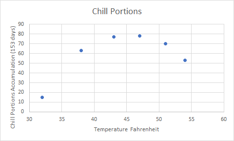
Figure 6. Chill portions accumulated for 153 days at a constant temperature. 153 days is the number of days between September 1st and February 1st.
Going back to the first chart (Figure 1), although Weather Station B has much lower temperatures than A, the temperature that it dips down to is in the suboptimal range (32 - 43 °F). At these times where Station B dips below Station A, Station B is accumulating less chill portions, but not fewer chill hours.
So next time you see large differences in chill hours between you, your neighbor, or your nearest regional weather station don’t be alarmed. It’s microclimate variation - and that is what we are here for!
Other Resources
The Almond Doctor: Counting Chill Better – Using the Chill Portions Model
UCANR: About Chilling Hours, Units & Portions
Related Posts
Semios: The Benefits of In-Canopy Weather Stations